May 7, 2021
0.0 Introduction
A health crisis of massive proportion such as the current COVID-19 pandemic has provided us ample opportunity to reflect on our healthcare system and how we can strengthen it. As we heard at the beginning of the pandemic, healthcare officials want to ‘flatten the curve’ to ensure sufficient supplies will be available to patients, thus minimizing casualties. For this report, I will look into data provided from COVID-19 patients, provided by the Mexican government (link), to build a model to predict hospitalization rates and hopefully provide insight on where to best allocate resources.
The dataset contains information on 566,602 patients for 23 different attributes. The original dataset uses 1's for yes, 2's for no, and (97,98,99, or 9999-99-99) for NA. Below, the bolded items are the attributes that remain in the report for analysis after cleaning, as the others either have a lot of NA's or 2's (no). I will tidy the data in Section 0.2 and begin analysis in Section 1.0.
id- unique number for patientssex- F/M (1/2)patient_type- not hospitalized/hospitalized (1/2)entry_date- date when patient entered hospitaldate_symptoms- date when patient started showing symptomsdate_died- date patient died (9999-99-99 means recovered)intubed- if patient needs ventilatorpneumonia- if patient has pneumoniaage- age of patientpregnancy- if patient is pregnantdiabetes- if patient has diabetescopd- if patient has Chronic Obstructive Pulmonary Disease (COPD)asthma- if patient has asthmainmsupr- if patient is immunosuppressedhypertension- if patient has hypertensionother_disease- if patient has another diseasecardiovascular- if patient had a history of a heart related diseaseobesity- if patient is obeserenal_chronic- if patient has chronic renal diseasetobacco- if patient uses tobacco productscontact_other_covid- if patient came in contact with someone else with covidicu- if patient was admitted to the ICUcovid_res- if patient has resistance - tested positive (1), negative (2), or is waiting for results (3)
0.1 Imports
library(tidyverse)

# import dataset
covid <- read.csv("covid.csv")
covid %>% head(3)
## id sex patient_type entry_date date_symptoms date_died intubed pneumonia
## 1 16169f 2 1 04-05-2020 02-05-2020 9999-99-99 97 2
## 2 1009bf 2 1 19-03-2020 17-03-2020 9999-99-99 97 2
## 3 167386 1 2 06-04-2020 01-04-2020 9999-99-99 2 2
## age pregnancy diabetes copd asthma inmsupr hypertension other_disease
## 1 27 97 2 2 2 2 2 2
## 2 24 97 2 2 2 2 2 2
## 3 54 2 2 2 2 2 2 2
## cardiovascular obesity renal_chronic tobacco contact_other_covid covid_res
## 1 2 2 2 2 2 1
## 2 2 2 2 2 99 1
## 3 2 1 2 2 99 1
## icu
## 1 97
## 2 97
## 3 2## remove id column
covid <- covid %>% select(-id)
# get number of rows
dim(covid)## [1] 566602 220.2 Tidying
0.2.1 Remove NAs
As mentioned above, the data provided uses 97, 98, and 99 to represent NA values. So the first step is to remove all occurrences of these numbers. I first remove columns that contain approximately >50% NA values (approximately >250,000 values), since they will mostly be removed anyways.
# step 1: remove all NA values (97, 98, 99)

## count NA-numbers (97, 98, 99) in dataset
count_na_nums <- function(x)sum(x==97 | x==98 | x==99)
covid %>% summarize_all(count_na_nums)
## sex patient_type entry_date date_symptoms date_died intubed pneumonia age
## 1 0 0 0 0 0 444813 11 207
## pregnancy diabetes copd asthma inmsupr hypertension other_disease
## 1 288699 1981 1749 1752 1980 1824 2598
## cardiovascular obesity renal_chronic tobacco contact_other_covid covid_res
## 1 1822 1781 1792 1907 175031 0
## icu
## 1 444814## remove features with lots of NA-numbers
covid <- covid %>%
select(-intubed,
-pregnancy,
-contact_other_covid,
-icu)I found that columns intubed, pregnancy, contact_other_covid, and icu have >50% NA values, so they are removed. Next, I will convert the all occurrences of 97-99 to NA_integer_ and then remove them using na.omit().
## convert NA-numbers to NA

## mutate if condition
has_na_num <-function(x)any(x==97 | x==98 | x==99)

## mutate if function (NA_integer_ to ensure T/F are of same type)
replace_num_na <- function(x)if_else((x==97 | x==98 | x==99), NA_integer_, x)

## replace values and remove
covid <- covid %>%
  mutate_if(has_na_num, replace_num_na) %>%
  na.omit()

## check for NA
covid %>% summarise_all( funs(sum(is.na(.))) )
## sex patient_type entry_date date_symptoms date_died pneumonia age diabetes
## 1 0 0 0 0 0 0 0 0
## copd asthma inmsupr hypertension other_disease cardiovascular obesity
## 1 0 0 0 0 0 0 0
## renal_chronic tobacco covid_res
## 1 0 0 0## see how mach data was lost
dim(covid)## [1] 562444 180.2.2 Create New Attributes
Since dates are difficult to analyze, I will create a new attribute incub_time, which is the time between a patient first notices symptoms (date_symptoms) and the date they checked into the hospital (entry_date).
# Step 2: create new numeric column for incubation time

# incub time = (hospital) entry date - symptom date
covid <- covid %>%
  mutate(incub_time = as.numeric(as.Date(entry_date, format="%d-%m-%Y") -
           as.Date(date_symptoms, format="%d-%m-%Y")) )

# check if worked
covid %>% select(entry_date, date_symptoms, incub_time) %>% head()
## entry_date date_symptoms incub_time
## 1 04-05-2020 02-05-2020 2
## 2 19-03-2020 17-03-2020 2
## 3 06-04-2020 01-04-2020 5
## 4 17-04-2020 10-04-2020 7
## 5 13-04-2020 13-04-2020 0
## 6 16-04-2020 16-04-2020 0# remove redundant columns
covid <- covid %>% select(-entry_date, -date_symptoms)I will also convert ages into the standard age ranges (<18, 18-29, 30-39, 40-49, 50-64, 65-74, and >75) to make future analysis easier and more meaningful. This data will become categorical with 7 categories.
# first make cut off ranges (case_when didn't work directly)
covid$age_cat <- cut(covid$age, breaks=c(0,18,30,40,50,65,75), right = FALSE)
covid$age_cat <- as.character(covid$age_cat)

# convert to more readable form
covid <- covid %>% mutate(age_range = case_when(
  age_cat == "[0,18)"  ~ "<18",
  age_cat == "[18,30)" ~ "18-29",
  age_cat == "[30,40)" ~ "30-39",
  age_cat == "[40,50)" ~ "40-49",
  age_cat == "[50,65)" ~ "50-64",
  age_cat == "[65,75)" ~ "65-74",
  TRUE ~ ">75"
))

# drop intermediate column
covid <- covid %>% select(-age_cat)

# view
covid %>% select(age, age_range) %>% head()
## age age_range
## 1 27 18-29
## 2 24 18-29
## 3 54 50-64
## 4 30 30-39
## 5 60 50-64
## 6 47 40-490.2.3 Convert to Binary
Next, I will convert the columns into their binary representations (0/1’s). Currently, they are entered as 1's for True/female and 2's for False/male. For example, for the columns diabetes, a 1 indicates that the patient has diabetes (True) and 2 indicates that the patient doesn’t have diabetes (False). This is true for all columns except for hospitalized, where the relationship is flipped for some reason. I will also convert the date_died to binary, where 0 is if the patient recovered (represented as 9999-99-99) and 1 is if the patient died (represented as an actual date). Lastly, I will convert the column covid_res to categorical data - positive, negative, waiting - for the values 1, 2, and 3 respectively, and rename the column to covid_test.
# step 3: convert to binary

## define functions
## 9999-99-99 = recovered (or 0); actual date == died (or 1)
change_date_to_binary <- function(x)if_else(x=='9999-99-99',0,1)

## 0 == F/Male; 1 == T/Female
# abs(2-2) = 0 (F/Male)
# abs(1-2) = 1 (T/Female)
change_nmbr_to_binary <- function(x)if_else(x<=2, abs(x-2), as.double(x))

## mutate
covid <- covid %>%
  # create covid_test categorical data
  mutate(covid_test = case_when(
    covid_res == 1 ~ "positive",
    covid_res == 2 ~ "negative",
    covid_res == 3 ~ "waiting")) %>%
  # convert `date_died` column to 0/1
  mutate_at(vars(date_died), change_date_to_binary) %>%
  mutate_at(vars(date_died), change_nmbr_to_binary) %>%
  # convert numeric columns to 0/1
  mutate_if(is.numeric, change_nmbr_to_binary) %>%
  # convert `sex` to M/F (0/1)
  mutate(sex = ifelse(sex == 0,'M','F')) %>%
  # switch 1/0 to 0/1 (not hospitalized/hospitalized) for `patient_type`
  mutate(hospitalized = ifelse(patient_type == 1,0,1)) %>%
  # rename columns
  rename(died = date_died) %>%
  # remove redundant column
  select(-patient_type, -covid_res)

# all clean up is done!
covid %>% head(3)
## sex died pneumonia age diabetes copd asthma inmsupr hypertension
## 1 M 0 0 27 0 0 0 0 0
## 2 M 0 0 24 0 0 0 0 0
## 3 F 0 0 54 0 0 0 0 0
## other_disease cardiovascular obesity renal_chronic tobacco incub_time
## 1 0 0 0 0 0 0
## 2 0 0 0 0 0 0
## 3 0 0 1 0 0 5
## age_range covid_test hospitalized
## 1 18-29 positive 0
## 2 18-29 positive 0
## 3 50-64 positive 10.2.4 Remove Attributes
For the last step, I will remove features that don’t have a large presence in the dataset. The dataset is very large and computation in the future sometimes doesn’t work on a local machine, so I will go ahead and prune the dataset now. I only remove features that have a mean of less that 10% (most columns are binary so the mean corresponds to the proportion of 1's). The 10% value was chosen arbitrarily.
# summarize all numeric columns (these are between 0 and 1)
colMeans(covid %>% dplyr::select(where(is.numeric)))
## died pneumonia age diabetes copd
## 0.06319029 0.15429447 42.56990918 0.12497778 0.01600515
## asthma inmsupr hypertension other_disease cardiovascular
## 0.03189829 0.01579002 0.16327137 0.03012744 0.02242890
## obesity renal_chronic tobacco incub_time hospitalized
## 0.16287488 0.01981886 0.08485111 3.70852209 0.21370661So, we see that copd, asthma, inmsupr, other_disease, cardiovascular, renal_chronic, and tobacco have means less than 0.10, so they will be removed. I will leave the column died as it will be a useful target variable.
covid <- covid %>% select(-copd,
                          -asthma,
                          -inmsupr,
                          -other_disease,
                          -cardiovascular,
                          -renal_chronic,
                          -tobacco)
dim(covid)
## [1] 562444 11Great! Now the data should be all cleaned up. Since there was a lot that changed, here is a new list of all attributes that are in the cleaned dataset. Most features should be binary (0/1), numeric, or character values.
sex- M/Fdied- if patient recovered/died (0/1)pneumonia- if patient does not have pneumonia/has pneumonia (0/1)age- numerical value of patient’s agediabetes- if patient does not have diabetes/has diabetes (0/1)hypertension- if patient does not have hypertension/has hypertension (0/1)obesity- if patient does not have obesity/has obesity (0/1)incub_time- days between start of symptoms and date checked into hospitalage_range- categories of age ranges (<18, 18-29, 30-39, 40-49, 50-64, 65-74, >75)covid_test- if patient’s covid test came out positive, negative, or is waitinghospitalized- if patient was not hospitalized/hospitalized (0/1)
0.2.5 Quick Stats
# quick stats on categorical data
# ratio of M/F
covid %>% group_by(sex) %>% summarise(n = round(n()/nrow(covid),2))
## # A tibble: 2 x 2
## sex n
## <chr> <dbl>
## 1 F 0.49
## 2 M 0.51# covid test
covid %>% group_by(covid_test) %>% summarise(n = round(n()/nrow(covid),2))## # A tibble: 3 x 2
## covid_test n
## <chr> <dbl>
## 1 negative 0.49
## 2 positive 0.39
## 3 waiting 0.12# age ranges
covid %>% group_by(age_range) %>% summarise(n = round(n()/nrow(covid),2))## # A tibble: 7 x 2
## age_range n
## <chr> <dbl>
## 1 <18 0.04
## 2 >75 0.04
## 3 18-29 0.18
## 4 30-39 0.24
## 5 40-49 0.22
## 6 50-64 0.21
## 7 65-74 0.061.0 Analysis of Variance
The pandemic has disproportionately been affecting the elderly population, due to the physiological changes that come with aging and potential pre-existing health conditions (ref). I would like to explore if the rates of pre-existing conditions do vary among the different age groups (as a check to see how accurate the data holds to the information we’ve heard). This can be examined through a multivariate analysis of variance test or a MANOVA test. I will compare the mean rates of pre-existing conditions - diabetes, hypertension, obesity - among different age groups (age_range).
H0: For each response variable, the means of all groups are equal (\(\mu_1 = \mu_2 = \ldots = \mu_m\)).
HA: For at least one response variable, at least one group mean differs (\(\mu_i \ne \mu_{i'}\)).
# MANOVA (1)
man <- manova(cbind(diabetes, hypertension, obesity)~age_range, data=covid)

# summary - statistical significance
summary(man)
## Df Pillai approx F num Df den Df Pr(>F)
## age_range 6 0.22251 7509.7 18 1687311 < 2.2e-16 ***
## Residuals 562437
## ---
## Signif. codes: 0 '***' 0.001 '**' 0.01 '*' 0.05 '.' 0.1 ' ' 1Since the p-value < 0.05, we can reject the null-hypothesis. Now, let’s find out which groups are different from each other for each variable.
# one way ANOVA (3 tests)
summary.aov(man)
## Response diabetes :
## Df Sum Sq Mean Sq F value Pr(>F)
## age_range 6 7481 1246.8 12980 < 2.2e-16 ***
## Residuals 562437 54027 0.1
## ---
## Signif. codes: 0 '***' 0.001 '**' 0.01 '*' 0.05 '.' 0.1 ' ' 1
##
## Response hypertension :
## Df Sum Sq Mean Sq F value Pr(>F)
## age_range 6 12695 2115.87 18553 < 2.2e-16 ***
## Residuals 562437 64142 0.11
## ---
## Signif. codes: 0 '***' 0.001 '**' 0.01 '*' 0.05 '.' 0.1 ' ' 1
##
## Response obesity :
## Df Sum Sq Mean Sq F value Pr(>F)
## age_range 6 1139 189.821 1413.2 < 2.2e-16 ***
## Residuals 562437 75548 0.134
## ---
## Signif. codes: 0 '***' 0.001 '**' 0.01 '*' 0.05 '.' 0.1 ' ' 1# pair-wised t-test (21 tests each)
pairwise.t.test(covid$diabetes, covid$age_range, p.adj="none")##
## Pairwise comparisons using t tests with pooled SD
##
## data: covid$diabetes and covid$age_range
##
## <18 >75 18-29 30-39 40-49 50-64
## >75 <2e-16 - - - - -
## 18-29 0.005 <2e-16 - - - -
## 30-39 <2e-16 <2e-16 <2e-16 - - -
## 40-49 <2e-16 <2e-16 <2e-16 <2e-16 - -
## 50-64 <2e-16 <2e-16 <2e-16 <2e-16 <2e-16 -
## 65-74 <2e-16 <2e-16 <2e-16 <2e-16 <2e-16 <2e-16
##
## P value adjustment method: nonepairwise.t.test(covid$hypertension,covid$age_range, p.adj="none")##
## Pairwise comparisons using t tests with pooled SD
##
## data: covid$hypertension and covid$age_range
##
## <18 >75 18-29 30-39 40-49 50-64
## >75 < 2e-16 - - - - -
## 18-29 7.4e-11 < 2e-16 - - - -
## 30-39 < 2e-16 < 2e-16 < 2e-16 - - -
## 40-49 < 2e-16 < 2e-16 < 2e-16 < 2e-16 - -
## 50-64 < 2e-16 < 2e-16 < 2e-16 < 2e-16 < 2e-16 -
## 65-74 < 2e-16 < 2e-16 < 2e-16 < 2e-16 < 2e-16 < 2e-16
##
## P value adjustment method: nonepairwise.t.test(covid$obesity, covid$age_range, p.adj="none")##
## Pairwise comparisons using t tests with pooled SD
##
## data: covid$obesity and covid$age_range
##
## <18 >75 18-29 30-39 40-49 50-64
## >75 < 2e-16 - - - - -
## 18-29 < 2e-16 < 2e-16 - - - -
## 30-39 < 2e-16 < 2e-16 < 2e-16 - - -
## 40-49 < 2e-16 < 2e-16 < 2e-16 < 2e-16 - -
## 50-64 < 2e-16 < 2e-16 < 2e-16 < 2e-16 1.9e-09 -
## 65-74 < 2e-16 < 2e-16 < 2e-16 < 2e-16 5.6e-06 < 2e-16
##
## P value adjustment method: noneFrom the one-way ANOVA tests and the individual t-tests, we see that most relations have differences in rates of pre-existing conditions between the various age groups (p < 0.05). However, it was interesting to see that the rates of diabetes between the age groups <18 and 18-29 are closer together than for other groups (p = 0.005).
That being said, since there were a lot of tests performed, we need to correct the p-value using the Bonferroni adjusted significance.
# n tests (1 MANOVA, 3 ANOVA, 63 t-tests)
X <- 1 + 3 + (3*21)

# prob of at least 1 type-I error
1 - 0.95^X
## [1] 0.9678277# Bonferroni adjusted significance level
0.05/X## [1] 0.0007462687The Bonferroni adjusted p-value is 0.0007. We see that the previous relation of diabetes between the age groups <18 and 18-29 is no longer significant. In other words, the mean rate of diabetes between the age groups <18 and 18-29 are similar.
# remove variable to clean environment
rm(list= ls()[!(ls() %in% c('covid','class_diag'))])
2.0 Randomization Test
From the MANOVA test we found that different age groups have different rates of pre-existing conditions (mostly). Now I would like to see how pre-existing conditions vary between men and women.
From some research and exploration of the dataset, I found that men are disproportionately affected by COVID-19 than women (ref). However, I would like to see if there is a significant different in pre-existing condition rates between the men and women who passed away to COVID-19.
# quick check

# isolate death cases
covid %>% filter(died == 1) %>%
  # nrow() = 35541
  group_by(sex) %>%
  summarise(death_rate = round(n()/35541, 3))
## # A tibble: 2 x 2
## sex death_rate
## <chr> <dbl>
## 1 F 0.352
## 2 M 0.648We see that of those who died, 65% were men and 35% were women.
2.1 Define Problem
To test to see if the rates of a pre-existing condition differ between men and women, I will perform a randomized test. First, I will look deeper into the three pre-existing conditions to see if men and women had similar rates for any one condition.
# filter dataset to only those who passed away
rnd_data <- covid %>% filter(died == 1)

# true mean pre-existing rates between M/F
rnd_data %>% group_by(sex) %>%
  summarise(diabetes_rate = mean(diabetes),
            hypert_rate = mean(hypertension),
            obesity_rate = mean(obesity))
## # A tibble: 2 x 4
## sex diabetes_rate hypert_rate obesity_rate
## <chr> <dbl> <dbl> <dbl>
## 1 F 0.420 0.494 0.270
## 2 M 0.341 0.382 0.215Interestingly, among those who passed away, women have higher rates of pre-existing conditions than men, even though men suffer more severe cases and die of COVID-19 than women. That must mean there are other factors that played a role in the outcomes of COVID-19 for men.
Since the obesity_rates are closest together, I will perform a randomized test on that pre-existing condition. This will provide us insight on how likely it is that obesity rates differ between the men and women who passed away from COVID-19.
2.2 Randomized Test
For the randomization test, I will shuffle the sex label and calculate the mean differences of obesity rates between the two groups.
H0: The average obesity rates among the two groups are equal.
HA: The average obesity rates among the two groups are not equal
# reduce dataset to important features
rnd_data <- rnd_data %>% select(sex, obesity)

# test
set.seed(813)

rand_dist <- vector()
for(i in 1:100){
  # sample sex
  perm <- data.frame(obesity=rnd_data$obesity,
                     sex=sample(rnd_data$sex))

  # mean difference (F - M)
  rand_dist[i] <- mean(perm[perm$sex=="F",]$obesity) -
                  mean(perm[perm$sex=="M",]$obesity)
}

# find true mean ages
orig_diff <- rnd_data %>% group_by(sex) %>%
  summarise(avg = mean(obesity)) %>%
  summarise(diff(avg)) %>% pull()
round(orig_diff, 3)
## [1] -0.055# p-value
mean(rand_dist < orig_diff | rand_dist > -orig_diff)## [1] 02.3 Null Distribution
# histogram
{hist(rand_dist, main="",ylab=""); abline(v = c(-orig_diff,orig_diff),col="red")}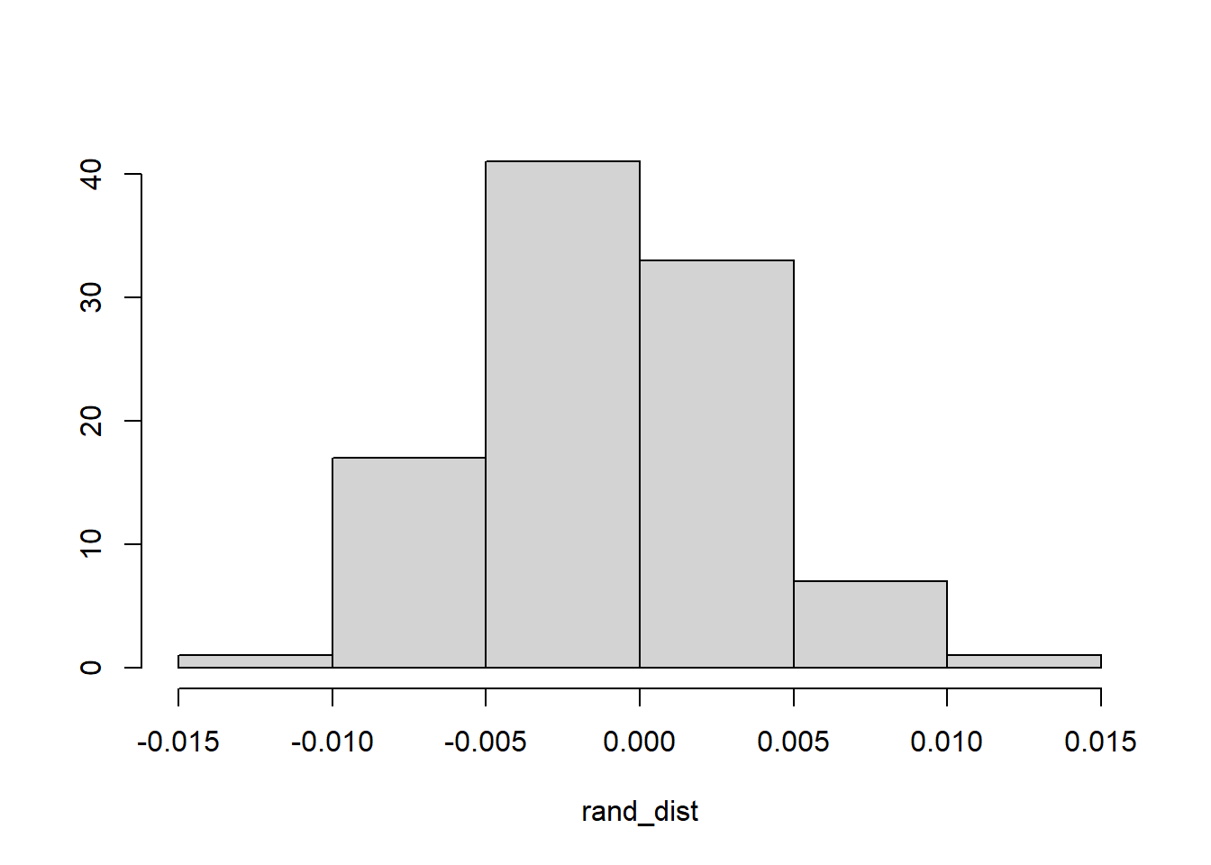
# orig_diff = -/+ 0.055From the randomized test, we see that there is no chance that the rates of obesity should vary so much between the men and women who passed away. The true mean difference in obesity rates between men and women is 0.055. However, the entire null distribution falls within -0.055 and +0.055.
# remove variable to clean environment
rm(list= ls()[!(ls() %in% c('covid','class_diag'))])
3.0 Linear Regression
3.1 Coefficients
Now I will build a linear regression model to predict the probability an individual will be hospitalized based on their sex and if they have any pre-existing conditions.
library(lmtest)
library(sandwich)

# linear regression model
lm_fit <- lm(hospitalized~sex*diabetes + sex*hypertension + sex*obesity,
             data=covid)
summary(lm_fit)
##
## Call:
## lm(formula = hospitalized ~ sex * diabetes + sex * hypertension +
## sex * obesity, data = covid)
##
## Residuals:
## Min 1Q Median 3Q Max
## -0.6329 -0.1882 -0.1133 -0.1133 0.8867
##
## Coefficients:
## Estimate Std. Error t value Pr(>|t|)
## (Intercept) 0.1132635 0.0008629 131.252 < 2e-16 ***
## sexM 0.0749031 0.0012167 61.562 < 2e-16 ***
## diabetes 0.2396085 0.0024833 96.489 < 2e-16 ***
## hypertension 0.1839564 0.0022128 83.134 < 2e-16 ***
## obesity 0.0137193 0.0020027 6.850 7.38e-12 ***
## sexM:diabetes 0.0162390 0.0033998 4.776 1.78e-06 ***
## sexM:hypertension -0.0123776 0.0030590 -4.046 5.21e-05 ***
## sexM:obesity 0.0035773 0.0028533 1.254 0.21
## ---
## Signif. codes: 0 '***' 0.001 '**' 0.01 '*' 0.05 '.' 0.1 ' ' 1
##
## Residual standard error: 0.3887 on 562436 degrees of freedom
## Multiple R-squared: 0.1008, Adjusted R-squared: 0.1008
## F-statistic: 9005 on 7 and 562436 DF, p-value: < 2.2e-16The intercept (0.113) indicates the probability of being hospitalized if you are a woman. As expected, men have a higher risk (+0.075) of being hospitalized. In general, all three pre-existing conditions increases an individuals risk of being hospitalized, however, diabetes and hypertension are more of a risk (0.240 and 0.184 respectively) than obesity (0.014). Diabetes and obesity increase the risk of being hospitalized for men specifically (0.016 and 0.004 respectively), however hypertension seems to reduce their risk.
3.2 Regression Plot
library(gridExtra)

# only plot 10% of data points (to reduce execution time)
set.seed(813)
plot_df <- sample_n(covid, 0.10*nrow(covid)) %>%
  select(sex, diabetes, hypertension, obesity, hospitalized)

# plot regressions
p1 <- qplot(diabetes, hospitalized, data=plot_df, color=sex) +
  geom_point() + geom_smooth(method='lm') +
  geom_vline(xintercept=mean(covid$diabetes,na.rm=T),lty=2)
p2 <- qplot(hypertension, hospitalized, data=plot_df, color=sex)+
  geom_point() + geom_smooth(method='lm') +
  geom_vline(xintercept=mean(covid$hypertension,na.rm=T),lty=2)
p3 <- qplot(obesity, hospitalized, data=plot_df, color=sex)+
  geom_point() + geom_smooth(method='lm') +
  geom_vline(xintercept=mean(covid$obesity,na.rm=T),lty=2)
grid.arrange(p1, p2, p3, nrow=3)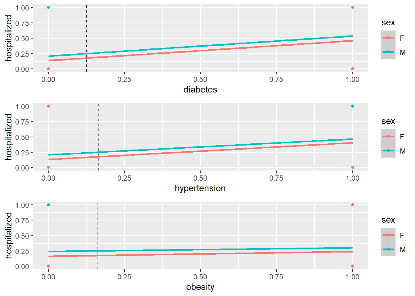
# R2
round(summary(lm_fit)$r.sq, 3)
## [1] 0.101The model explains about 10.1% of the variation in the outcomes.
3.3 Check Assumptions
# check assumptions of linearity, normality, homoscedasticity
bptest(lm_fit)
##
## studentized Breusch-Pagan test
##
## data: lm_fit
## BP = 26951, df = 7, p-value < 2.2e-16# Corrected SE
coeftest(lm_fit, vcov=vcovHC(lm_fit))##
## t test of coefficients:
##
## Estimate Std. Error t value Pr(>|t|)
## (Intercept) 0.11326353 0.00072028 157.2496 < 2.2e-16 ***
## sexM 0.07490312 0.00112699 66.4631 < 2.2e-16 ***
## diabetes 0.23960855 0.00306430 78.1936 < 2.2e-16 ***
## hypertension 0.18395645 0.00262269 70.1403 < 2.2e-16 ***
## obesity 0.01371925 0.00203550 6.7400 1.586e-11 ***
## sexM:diabetes 0.01623897 0.00424710 3.8235 0.0001316 ***
## sexM:hypertension -0.01237764 0.00371066 -3.3357 0.0008509 ***
## sexM:obesity 0.00357732 0.00309180 1.1570 0.2472575
## ---
## Signif. codes: 0 '***' 0.001 '**' 0.01 '*' 0.05 '.' 0.1 ' ' 1Based on the Breusch-Pagan test, the p-value < 0.05, indicating that we can reject the null hypothesis and that too much of the variance is explained by additional explanatory variables (heteroscedasticity). There are minimal changes in the SE. Some features, like interecept and sexM`, the corrected SE was reduced. For the remaining features, the corrected SE was increased.
# remove variable to clean environment
rm(list= ls()[!(ls() %in% c('covid','class_diag'))])
4.0 Bootstrapping
Now, I will compute the bootstrapped SE for the regression model found in Section 3.0.
# select important datapoints
dat <- covid %>% select(sex, diabetes, hypertension, obesity, hospitalized)

# bootstrap SE of slope (re-sampling observations)
set.seed(813)

# there is a lot of data, so I will only do 100 samples
# though, I get the same results for 100 and 5000 samples
samp_distn <- replicate(100, {
  boot_dat <- sample_frac(dat, replace=T)
  fit <- lm(hospitalized~sex*diabetes + sex*hypertension + sex*obesity,
            data=boot_dat)
  coef(fit)
})

# compare the two methods
samp_distn %>% t %>% as.data.frame %>% summarise_all(sd)
## (Intercept) sexM diabetes hypertension obesity sexM:diabetes
## 1 0.0008029077 0.00116445 0.002883634 0.002639915 0.002122281 0.003962536
## sexM:hypertension sexM:obesity
## 1 0.004055147 0.002799329The all bootstrapped SE except for sexM:obesity are slightly higher than the SE found in Section 3.1. All SE, except for sexM:obesity were statistically significant in Section 3.1, so the respective bootstrapped SE should also be statistically significant.
# remove variable to clean environment
rm(list= ls()[!(ls() %in% c('covid','class_diag'))])
5.0 Logistic Regression - Subset of Data
Although the linear regression provided some meaningful feedback from the coefficiets we fitted, a logistic regression would be much more effective for this dataset, since most features are binary. I will re-fit a logistic regression model on the same features from the linear regrssion model.
5.1 Coefficients
# logistic regression
glm_fit <- glm(hospitalized~sex*diabetes + sex*hypertension + sex*obesity,
               data=covid, family="binomial")
exp(coef(glm_fit))
## (Intercept) sexM diabetes hypertension
## 0.1315540 1.7798828 3.4450146 2.8544815
## obesity sexM:diabetes sexM:hypertension sexM:obesity
## 1.1078153 0.9226426 0.7992492 0.9946613The coefficients indicate that sexM, diabetes, and hypertension all increase the risk of being hospitalized by a factor of 1.77. 3.44, and 2.85 respectively. The features sexM:hypertension reduces the risk of being hospitalized by a factor of 0.799. The remaining features don’t seem impact your risk of being hospitalized by the coronavirus (~1).
5.2 Confusion Matrix
Let’s see how well the model performed.
# confusion matrix
prob <- predict(glm_fit, type="response")
pred <- ifelse(prob>.5,1,0)
table(truth=covid$died, prediction=pred) %>% addmargins
## prediction
## truth 0 1 Sum
## 0 497642 29261 526903
## 1 27380 8161 35541
## Sum 525022 37422 562444# acc, tpr, tnr, ppv, auc
class_diag(prob, covid$died)## acc sens spec ppv auc
## 1 0.8992949 0.2296221 0.9444661 0.2180803 0.7350419It looks like the model was about 90% accurate in predicting if an individual would be hospitalized by the coronavirus based on inputs like their sex and pre-existing conditions. The AUC is about 0.74.
5.3 Density Plot
# log-odds
covid$logit <- predict(glm_fit, type="link")

covid %>% ggplot()+
  geom_density(aes(logit, color=hospitalized, fill=hospitalized), alpha=.4)+
  theme(legend.position=c(.85,.85))+
  geom_vline(xintercept=0)+
  xlab("logit (log-odds)")+
  geom_rug(aes(logit,color=hospitalized))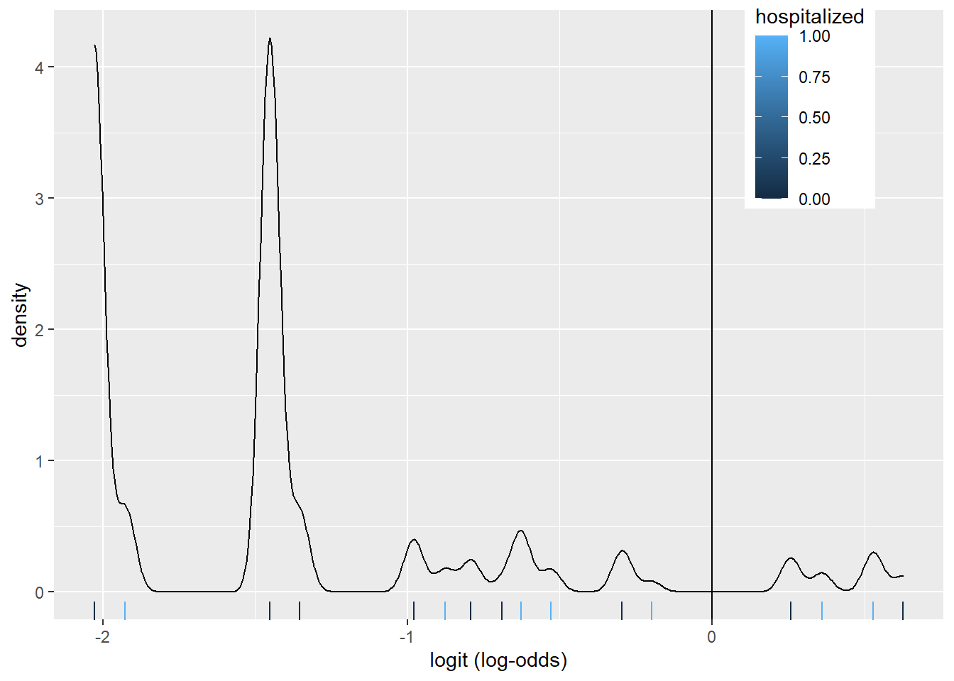
The density plot looks a little busy, but that might be due to fact that we fit a logistic regression model on many factors and interactions. There are about 8 pairs of density plots, one for each feature from the model. They can be seen better when we color the density plots by sex.
covid %>% ggplot()+
  geom_density(aes(logit, color=sex, fill=sex), alpha=.4)+
  theme(legend.position=c(.85,.85))+
  geom_vline(xintercept=0)+
  xlab("logit (log-odds)")+
  geom_rug(aes(logit,color=sex))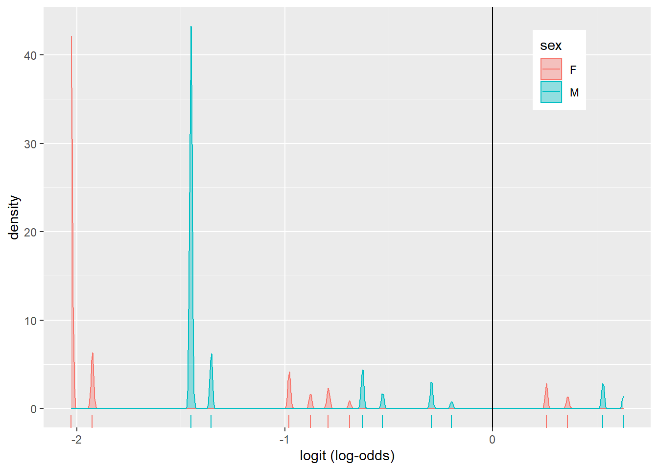
5.4 ROC, AUC Curves
library(plotROC)

# ROC plot
ROCplot <- ggplot(covid) + geom_roc(aes(d=died, m=prob), n.cuts=0)
ROCplot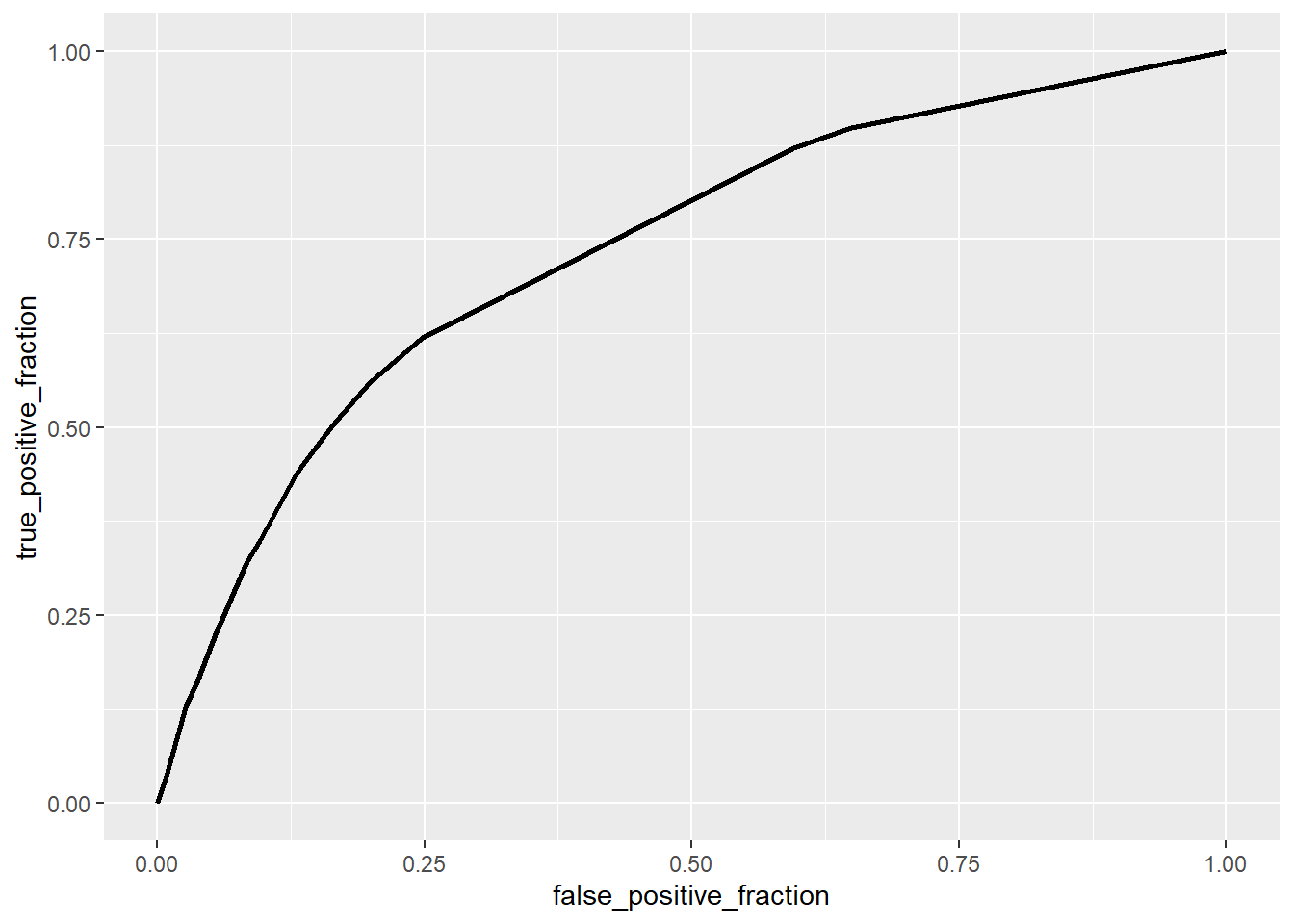
# AUC
calc_auc(ROCplot) %>% select(AUC) %>% pull()
## [1] 0.7350419The area under the curve is about 0.74, meaning that the degree of separability between being hospitalized and not hospitalized is about 74%.
# remove variable to clean environment
rm(list= ls()[!(ls() %in% c('covid','class_diag'))])
6.0 Logistic Regression - All of Data
Now I will perform a logistic regression on all the attributes
6.1 Fit Model
# remove age since it is redundant with age_range
covid <- covid %>% select(-age, -died)

glm_fit2 <- glm(hospitalized~., data=covid, family="binomial")
exp(coef(glm_fit2))
## (Intercept) sexM pneumonia diabetes
## 0.3452204 1.1241626 33.0892376 1.1711701
## hypertension obesity incub_time age_range>75
## 0.9603159 1.0121086 0.9889418 1.8754025
## age_range18-29 age_range30-39 age_range40-49 age_range50-64
## 0.2038129 0.2265116 0.3394530 0.5941156
## age_range65-74 covid_testpositive covid_testwaiting logit
## 1.2744252 1.7112068 1.4327928 1.5380026# predict outcome using fitted model
prob <- predict(glm_fit2, type="response")
# acc, tpr, tnr, ppv, auc
class_diag(prob, covid$hospitalized)## acc sens spec ppv auc
## 1 0.8897864 0.6125892 0.9651257 0.8268149 0.8843586With all the features, the model has about the same accuracy (0.89) as the previous logistic regression model (0.90). However, the AUC is much higher (0.88) than the previous model’s AUC (0.74).
6.2 10-Fold CV
# k-folds
set.seed(813)
k = 10 # number of folds

data<-covid[sample(nrow(covid)),] #randomly order rows
folds<-cut(seq(1:nrow(covid)), breaks=k, labels=F) #create folds

diags<-NULL
for(i in 1:k){
  ## Create training and test sets
  train<-data[folds!=i,]
  test<-data[folds==i,]

  truth<-test$hospitalized

  ## Train model on training set (all but fold i)
  fit<-glm(hospitalized~.,data=train,family="binomial")

  ## Test model on test set (fold i)
  probs<-predict(fit, newdata = test,type="response")

  ## Get diagnostics for fold i
  diags<-rbind(diags,class_diag(probs,truth))
}

summarize_all(diags,mean)
## acc sens spec ppv auc
## 1 0.8898059 0.6126758 0.9651306 0.8268423 0.8843456The 10-fold CV on the dataset with all attributes as about the same AUC (0.88) as the previous AUC value. This indicates that the model is not over-fitting.
6.3 LASSO
Although the model is not over-fitting, I would like to see which features the model deems important. So, I will perform a LASSO regression on the same model.
# LASSO
library(glmnet)
set.seed(813)

# lasso regression
covid_x <- model.matrix(hospitalized~., data= covid)[,-1]
covid_y <- as.matrix(covid$hospitalized)

## scale x
covid_x <- scale(covid_x)

# remove dataset - so lasso can fit in memory
rm(covid)

## lasso
cv.lasso1 <- cv.glmnet(x=covid_x, y=covid_y, family="binomial")
lasso1 <- glmnet(x=covid_x, y=covid_y, family="binomial", alpha=1,
                 lambda=cv.lasso1$lambda.1se)
coef(lasso1)
## 16 x 1 sparse Matrix of class "dgCMatrix"
## s0
## (Intercept) -1.77229732
## sexM 0.05245697
## pneumonia 1.24487665
## diabetes 0.05195450
## hypertension .
## obesity .
## incub_time -0.01894819
## age_range>75 0.18243150
## age_range18-29 -0.45409861
## age_range30-39 -0.47208513
## age_range40-49 -0.29058618
## age_range50-64 -0.06006259
## age_range65-74 0.13537974
## covid_testpositive 0.22887987
## covid_testwaiting 0.08795848
## logit 0.26732409The LASSO indicates that only obesity does not help with improving the model’s predictions.
6.4 10-Fold CV on LASSO Selected Featuers
# re-read covid data
covid <- read.csv("covid_sm.csv")

# remove feature with LASSO of 0
lasso_dat <- covid %>% select(-obesity)

# redo 10-fold CV with new dataset
set.seed(813)
k=10

data1<-lasso_dat[sample(nrow(lasso_dat)),] #put dataset in random order
folds<-cut(seq(1:nrow(lasso_dat)),breaks=k,labels=F) #create folds

diags<-NULL
for(i in 1:k){
  # train and test datasets
  train<-data1[folds!=i,]
  test<-data1[folds==i,]

  truth<-test$hospitalized

  ## Train model on training set (all but fold i)
  fit<-glm(hospitalized~., data=train,family="binomial")

  ## Test model on test set (fold i)
  probs<-predict(fit, newdata = test,type="response")

  ## Get diagnostics for fold i
  diags<-rbind(diags,class_diag(probs,truth))
}

# average the diagnostics for all k-folds
summarize_all(diags,mean)
## acc sens spec ppv auc
## 1 0.8996167 0.6547846 0.9661594 0.840225 0.8927561Lastly, the final 10-fold CV after LASSO has the same (but slightly better) AUC of 0.89. Again, this indicates that the model did not over-fit.
## R version 4.0.3 (2020-10-10)
## Platform: i386-w64-mingw32/i386 (32-bit)
## Running under: Windows 10 x64 (build 19041)
##
## Matrix products: default
##
## locale:
## [1] LC_COLLATE=English_United States.1252
## [2] LC_CTYPE=English_United States.1252
## [3] LC_MONETARY=English_United States.1252
## [4] LC_NUMERIC=C
## [5] LC_TIME=English_United States.1252
##
## attached base packages:
## [1] stats     graphics  grDevices utils     datasets  methods   base
##
## other attached packages:
##  [1] glmnet_4.1-1    Matrix_1.2-18   plotROC_2.2.1   gridExtra_2.3
##  [5] sandwich_3.0-0  lmtest_0.9-38   zoo_1.8-9       forcats_0.5.1
##  [9] stringr_1.4.0   dplyr_1.0.5     purrr_0.3.4     readr_1.4.0
## [13] tidyr_1.1.3     tibble_3.1.1    ggplot2_3.3.3   tidyverse_1.3.1
##
## loaded via a namespace (and not attached):
##  [1] httr_1.4.2        sass_0.3.1        jsonlite_1.7.2    splines_4.0.3
##  [5] foreach_1.5.1     modelr_0.1.8      bslib_0.2.4       assertthat_0.2.1
##  [9] highr_0.9         cellranger_1.1.0  yaml_2.2.1        pillar_1.6.0
## [13] backports_1.2.1   lattice_0.20-44   glue_1.4.2        digest_0.6.27
## [17] rvest_1.0.0       colorspace_2.0-1  htmltools_0.5.1.1 plyr_1.8.6
## [21] pkgconfig_2.0.3   broom_0.7.6       haven_2.4.1       bookdown_0.22
## [25] scales_1.1.1      mgcv_1.8-35       generics_0.1.0    farver_2.1.0
## [29] ellipsis_0.3.2    withr_2.4.2       cli_2.5.0         survival_3.2-11
## [33] magrittr_2.0.1    crayon_1.4.1      readxl_1.3.1      evaluate_0.14
## [37] ps_1.6.0          fs_1.5.0          fansi_0.4.2       nlme_3.1-152
## [41] xml2_1.3.2        blogdown_0.20     tools_4.0.3       hms_1.0.0
## [45] lifecycle_1.0.0   munsell_0.5.0     reprex_2.0.0      compiler_4.0.3
## [49] jquerylib_0.1.4   rlang_0.4.10      grid_4.0.3        iterators_1.0.13
## [53] rstudioapi_0.13   labeling_0.4.2    rmarkdown_2.8     codetools_0.2-18
## [57] gtable_0.3.0      DBI_1.1.1         R6_2.5.0          lubridate_1.7.10
## [61] knitr_1.33        utf8_1.2.1        shape_1.4.5       stringi_1.5.3
## [65] Rcpp_1.0.5        vctrs_0.3.8       dbplyr_2.1.1      tidyselect_1.1.1
## [69] xfun_0.22
## [1] "2021-05-17 15:23:08 CDT"## sysname release version nodename machine
## "Windows" "10 x64" "build 19041" "VIGGY" "x86"
## login user effective_user
## "viggy" "viggy" "viggy"